An advanced data analysis of empirical data for one variable. Histogram.
The advance analysis of the experiment of measurement of one variable is explained. If the variable has unknown nature the best way to get most complete presentation of the experiment is obtaining function of probability distribution and for simulating its behavior inverse probability distribution. To get these functions histogram of data set from experiment can be used.
The article A basic data analysis of the one variable. explains how to extract most general information from set of values these obtain for characteristic of one parameter of experiment or observation in nature. Here we will go much dipper compare to ordinary calculation of average and standard deviation. It is important also to emphasize here that methods describe below are completely separate from any assumption about structure or limitations of data to analyze. We are talking about output of so named black box. It gives to researcher one number after another and that is all what we have for analysis here.
If one measures the same parameter many times and have array of values the questions for elementary, basic analysis are what is the most probable value for next act of measurement and what the most probable deviation of that next measurement would be from this most probable value. It is valuable information to have but far from complete that can be obtained in theory if budget for research is big enough.
Let's illustrate the situation with the challenge to reproduce results of the unknown function that outputs random numbers. To be exact the function is constructed by author and known to him but we will pretend that it is forgotten after series of calculations. The task is to be able redone such series with properties as close to initial as possible. We will calculate 5 series of random numbers with the help of this function and save them in some file.
| N points | Average | σ, Standard deviation | Min | Max |
| 10 | 4.747 | 1,576 | 2,26 | 6,82 |
| 100 | 4.094 | 1.293 | 2 | 7.09 |
| 1000 | 4.07 | 1.35 | 1.74 | 8.08 |
| 10000 | 4.114 | 1.394 | 1.17 | 9.43 |
| 100000 | 4.104 | 1.391 | 1.06 | 9.62 |
At the first sign there is no qualitative difference between statistical characterization of these series no matter how many points are included in each of them. One can stop analysis at this point and report that answer is 4.1 ± 1.4 with likely normal distribution of points. It is most of what basic data analysis can do.
What if the problem is not just intellectual excise but has significant consequences. What if you will be offered to make the bet that next point will be inside interval with width equal to one. What interval would you choose to have best chances to win the bet? Naive answer would be the interval from 3.6 to 4.6 that is located around average value. This would be wrong in presented case.
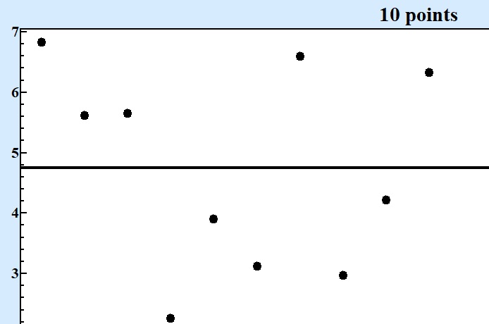
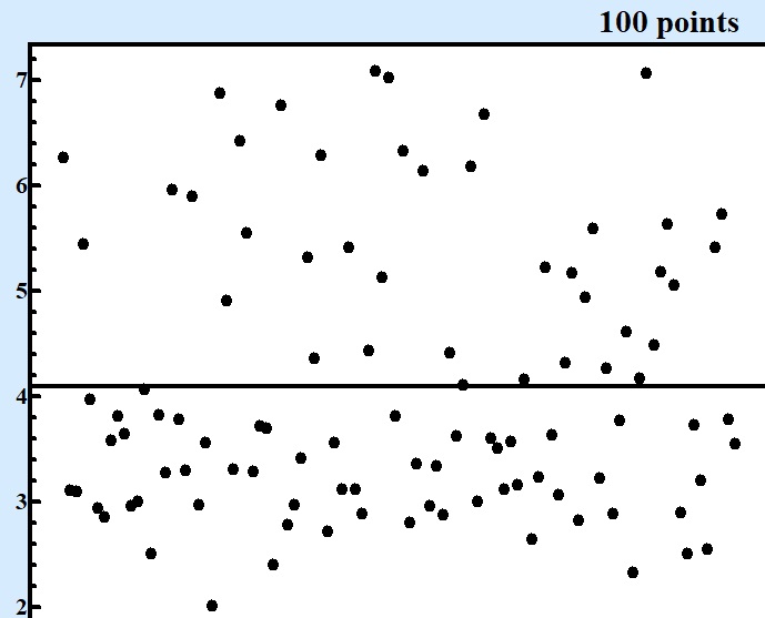
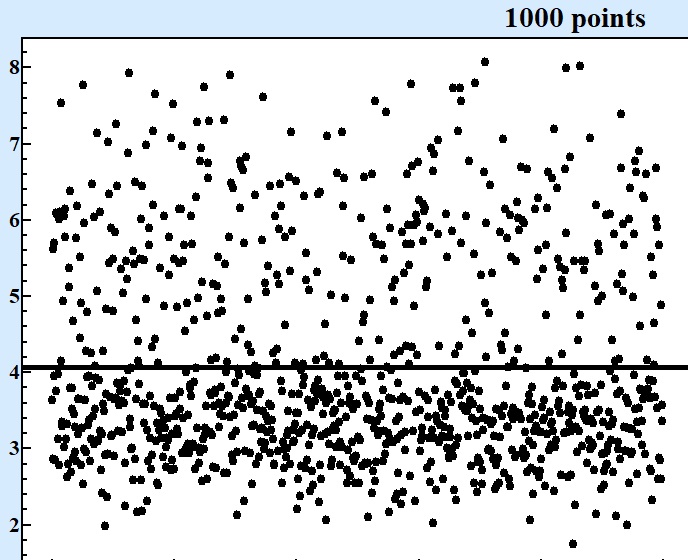
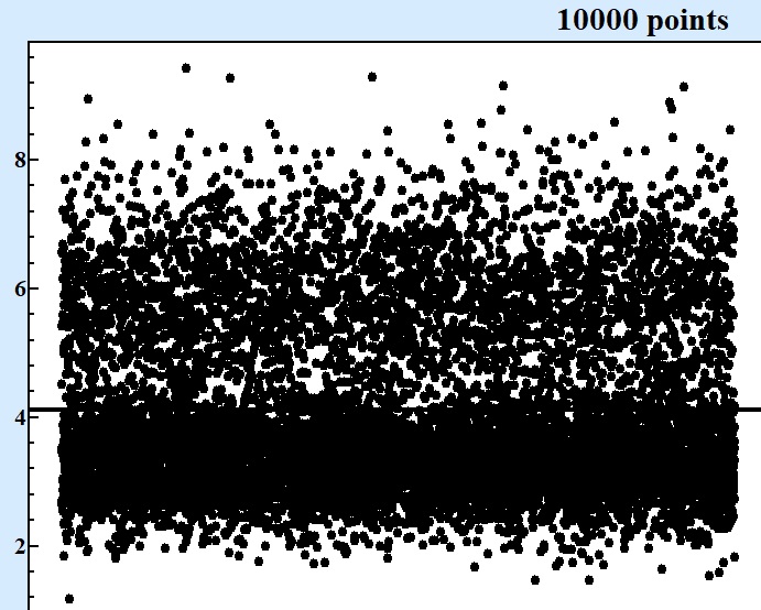
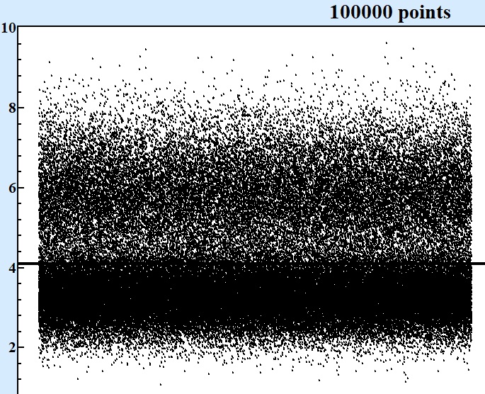
At Fig.1 these five series in questions are displayed at charts displaying of consecutive points in each series:
|
|
|
|
|
Fig. 1 Series of numbers of various size produced by the same random formula. |
Only starting from series contained 10000 points and more it becomes clear that there are at least two areas around values 3 and 6 where concentration of points are larger. For series with 1000 points one can see asymmetry of random values but cannot be sure that there is valley around 4.5.
Although presentation of results by consequent points on the chart as at Fig.1 can show the qualitative picture where next point most possible to fall but it adds very little in answering to the question about the best bet with precision that can give competitive advantage. Looking at Fig. 1 with 100000 points one can state for sure that interval between 2.7 and 3.7 will be good bet.
Let's fantasize that you can attract gamblers to make bets on interval where next point will be. The rules will be like this - gambler is choosing interval, any interval on the numerical axis and you as dealer will give him the odds of winning: 1 to x. Then gambler does agree and placing the bet or not. You as dealer of the game want to give gamblers an average payout somewhere about 93% as historically all successful casinos learned to do for keeping gamblers hope alive and in the same time to have reliable profit on the long run.
In principle it is quite simple task. One can take series of points produced by this random formula and calculate how many points are inside any given interval, then divide on number of all points in the series that will give a probability of any next point to be in that interval. Invert value is exact value of neutral odd for the bet. Neutral odd means that nobody has no advantage no gamble neither dealer. Multiplying the neutral odd on desired payout obtaining the odd to present to gambler.
| Interval | Points inside | Part of all points | Neutral odds |
Odds to set
Neutral odds*payout (0.93) |
| 3.6 - 4.6 | 20066 | 0.20066 | 1 : 4.989024147 | 1 : 4.639792457 |
| 2.7 - 3.7 | 44274 | 0.44274 | 1 : 2.258661969 | 1: 2.100555631 |
Of course in real life you would round odds to the closest, in your favor, presentation in form of rational fractions. For 3.6 - 4.6 interval odds to give is 2 : 9 and for interval 2.7 - 3.7 odds to be 1 : 2.
Interesting that if you as gambler would limit yourself with only basic analysis of series you would consider the first option to bet on interval around average so much more attractive compare all other options. In fact all gamblers on the long run will lose money at approximately the same pace because casino makes not basic but advance analysis. The behavior of gamblers is much complex problem than data analysis even advance one. It is more about physiology and physiology producing hormones in of stress situation than cold calculation of mathematical expectations, the high win often is more lucrative compare to better payout on long run because thought about . This fascinating issue is out of the scope of this article.
The method of defining probability of next point to be inside given interval described above by counting such points in big series is in fact correct one and plus the basic for any other analysis. It is of course too cumbersome and ugly too make count every time when interval in question is changed. Ironically with progress in computation power finding elegant mathematical solutions could be unpractical as soon it could be no noticeable difference between nanosecond of calculation of some sophisticated formula that need months of hard work of mathematician to develop or microsecond to direct count points in series. For some life problems simple counting could be rational approach but to get any sort of understanding of nature of random number source (to learn what black box has inside) one need to dig deeper.
The function of probability distribution gives complete information about random variable. In some sense any variable can be considered to be random because limited precision of any measurement. One can completely relay on function of probability distribution for description of behavior of one variable. If this function is precisely correct... that is impossible to know in principle because any number of experiments are limited in size. Here is fundamental vicious circle. No matter how many measurements are performed any additional one will improve precision of the experiment as a whole. There is no limits the process of measurement and any time could be surprise. You can switch on a lamp thousand times and think that there is iron clad connection between putting switch on and lighting until someday can be blackout or lamp burned out. There is no such thing as perfect final experiment.
The straightforward way of obtaining probability distribution goes through building a histogram. There are following steps are needed to create histogram from series of points:
- Find minimum and maximum values in series of measurements.
- Divide interval between minimum and maximum values into N equal intervals, so named bins.
- Count how many points in series are falling in each bin.
- Display each bin on the chart as rectangle with height proportional to number points in it.
Each of steps above deserves additional discussion and clarifications. A theoretical domain of possible values of any physical variable is from minus infinity till positive infinity. When we have series of points found minimum and maximum are not necessary and most possible are not borders of actual domain of the variable. The more points in series the better chance that interval of values will be larger. There is no harm in reasonable spreading limits of interval when building histogram.
A chose number of bins in interval when building histogram is a matter of balance between two conflicting considerations. The more bins (subintervals) the better resolution of probability function. If the variable gives a noise like signal thus there could be spikes in narrow interval of values so they are easy to be missed when subintervals are too large. Otherwise if subintervals are so small that most of them contain only several points there is no advantage in defining function of probability. We are using following formula for defining number of bins for building histogram:
Nbins = 3 * log10(Npoints) (1)
where Npoints - whole number points on series, Nbins - number intervals in histogram rounded to integer, log10 - logarithm with base 10. For practical situation some shifting of bin positions to put borders to round integers and rational fractions could be helpful from esthetical view and no or little effect on the analysis.
Returning to our example the Fig. 2 shows a histogram for the series in 100000 points:
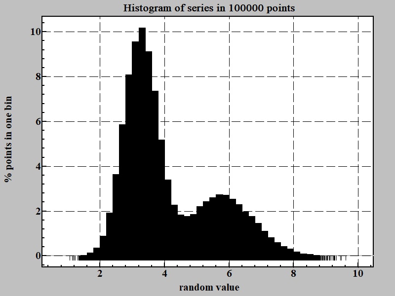
It is obvious from histogram above that there are at least two sources for random numbers in function producing series. One with maximum around 3.2 and other somewhere at 5.7.
Our software LeoDataAnalysis can help nor only in building histogram like displayed at Fig. 2 but also permits in some common cases to find probability distribution in form of function by following steps after obtaining reliable looking histogram. At tab "Results" push button "Report" then paste it into spreadsheet like MS Excel. Selecting two columns in report - value of bin and percent of points one can create and transfer series P(n) and fit them with incorporated into LeoDataAnalysis peaks search algorithm. Result of this procwdure is shown at Fig. 3:
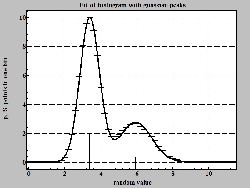
The fitting formula can be presented in following form as sum of two Gaussian functions:
p = ∑ 0.399*(A/σ)*exp(-0.5*( x-x)/σ)2)
p = 0.399*((13.55/0.528)*exp(-0.5*((v-3.35)/0.528)^2)+(6.17/1.004)*exp(-0.5*((v-5.86)/1.004)^2))
It brings us to the following hypothesis about nature of the data source: two random functions with Gaussian like distribution that can be characterized by point of maximum probability and standard deviation from it:
ni = x ± σ (1)
in our case n1 = 3.35 ± 0.528 and n2 = 5.86 ± 1.004
There is practically important property of Gaussian function that defines integral of it in whole arithmetical domain from minus to plus infinity to be equal A:
It means that a ratio of weights Gaussian like random sources is proportional to A. In our case number of points produced by first random source is A1/(A1+A2) = 13.55/(13.55+6.17) = 0.687 = 68.7 % and weight of second is 1- 0.687 = 0.313 = 31.3 %
The analysis above has very good agreement with the random formula that is timed to be be revealed:
ni = 1+rand(0.5)+if(rand(1)-0.66,2+gauss(0.5),10,4.5+gauss(1)) (2)
where rand(x) - function producing random number uniformly distributed from 0 till x; gauss(x) - a function producing random number distributed proportionally Gaussian function with maximum at 0 and standard deviation equal x; if(cond,f<0,f==0,f>0) - conditional function that depend on value of first argument to be less, equal or more than zero produces corresponding second, third or forth argument as output. According of the structure of formula (2) it should with probability 34% output Gaussian random number n1 = 3.25 ± 0.5 and with probability 66% Gaussian n2 = 5.75 ± 1. Analysis above gives us very good agreement with hidden formula.
But what to do if there is no reasonable simple formula behind data set but we need to reproduce its random numbers output of as close to observed series as possible? Or what to do if there is no random functions like gauss(x), only standard rand() uniformly distributed from 0 to 1, in your disposal but nevertheless you want reproduce random results?
Cumulative distribution function.
Fig.4 shows cumulative distribution functions for discussed above series.
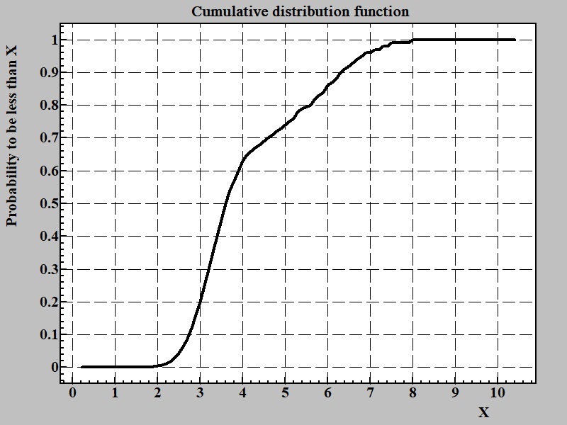
Cumulative distribution function gives probability that random variable will have value less than any give one. There is straightforward procedure to get cumulative function from histogram. Number points in each bin in histogram is consequentially summing from most left (corresponding to smallest value of the random variable) till very right (largest). Other way to formulate the same rule is to say that number of points in each bin is sum of all points in all bins with values less of equal to the given bin.
The cumulative distribution function has very helpful property - difference of its values for two given numbers is probability for the point to be inside interval between these two points. Thus an obtaining of cumulative probability function is the ultimate solution for the problem formulated above about calculating neutral bet in a game of guess. The most difficult aspect of using cumulative distribution function is obtaining it in analytical form that is easy to calculate. For example calculating trust interval for T-distribution (Student distribution) up to some time decades ago was tout to university students to be done via precalculated tables (like logarithms were). In spite that there is analytical algorithm for calculation of trust interval of Student distribution before personal computers a time to calculate even one value was way to long compare usage of the table.
In general case of empirical analysis of random variable the usage of cumulative distribution after collecting big enough experimental points from cumulative histogram is build and array of points [x,Px<0]i, where Px<0 - probability of the random value to be less than x. To get Px<0 for any given value one can use linear interpolation with base of two most closest points in array one of them lower and other is higher of the examined point.
If the task at hand to mimic behavior of random variable obtaining the inverse cumulative function is the way to go. The inverse cumulative function:
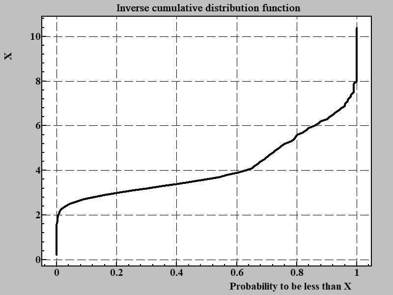
A domain of argument of inverse cumulative distribution function is between 0 and 1.0 This function is instrumental tool for coding random numbers function with probability distribution obtained from experiment. In some way inverse distribution function can be considered as modulator of uniformly distributed random number source into associated with this particular implementation of it. If N0→1 is inverse distribution function with argument that is defined between 0 to 1 and rand() - function producing uniformly distributed number in this interval (0 → 1). The function N0→1(rand()) will produce random numbers with given probability distribution.
Summary.
The ultimate result of experiment for measuring one variable is detailed as possible distribution probability function.
The distribution probability function can be obtained by building histogram.
Inverse distribution function is direct source for calculation probabilities of the variable to be inside any given interval during next measurement and also permits to modulate uniformly distributed variable into random variable mimicking obtained from experiment.
Apr. 7, 2018; 12:44 EST